Sampling arbitrary probability distributions
Transforming a uniform distribution to an arbitrary probability distribution
The universe we live in is, to the best of our (current) computational capabilities, wildly non-deterministic. Until the advent of computers, any desire for determinism had to be sated with the imagination, by defining and manipulating mathematical objects. Then came along machines that enabled us to specify processes that would carry on with unprecedented determinism, and we loved it. But even in those machines we couldn’t do without a sprinkle of non-determinism, so we added pseudorandom number generators and true random number generators (and also this).
Manipulating randomness
While most programming languages provide primitives for sampling from random distributions, sampling from your distribution of choice might require some work.
For example, C has rand() which generates an integer between 0 and RAND_MAX. To generate an integer within the constrained range (min, max) we use
rand() % (max - min + 1) + min. This is a trivial example, but it wasn’t trivial to me when I first learned it, and the fascination with transforming random numbers has stuck.
Many languages and libraries provide functions for sampling non-uniform distributions, such as the normal distribution. These functions all rely on a source of uniform random numbers,
and use some method to convert the uniform distribution to the desired distribution. One of the most general methods to convert uniformly-generated numbers in the range [0, 1]
to any probability distribution (both discrete and continuous) is inverse transform sampling.
We’ll get to how it works right after the fun part.
The fun part
This is actually the reason for the post. Here you can draw whatever discrete probability distribution you like, and sample from it! Just draw like in a paint program (the dynamic is a bit different because we’re drawing a function). You can choose from several initial distributions. (This part is best viewed on desktop).
0
Inverse transform sampling
Let’s develop the idea behind this sampling technique.
First, suppose you want to randomly select one out of four objects, A, B, C, D, uniformly. Easy: just sample a uniform random number in the range [0, 1].
If it’s between 0 and 0.25, select A; if it’s between 0.25 and 0.5, select B; etc.
Now suppose we have different probabilities for each object, for example A: 0.7, B: 0.2, C: 0.08, D: 0.02. Again we can use a uniform random number; if it’s between
0 and 0.7, select A; if it’s between 0.7 and 0.9, select B; if it’s between 0.9 and 0.98, select C; otherwise select D.
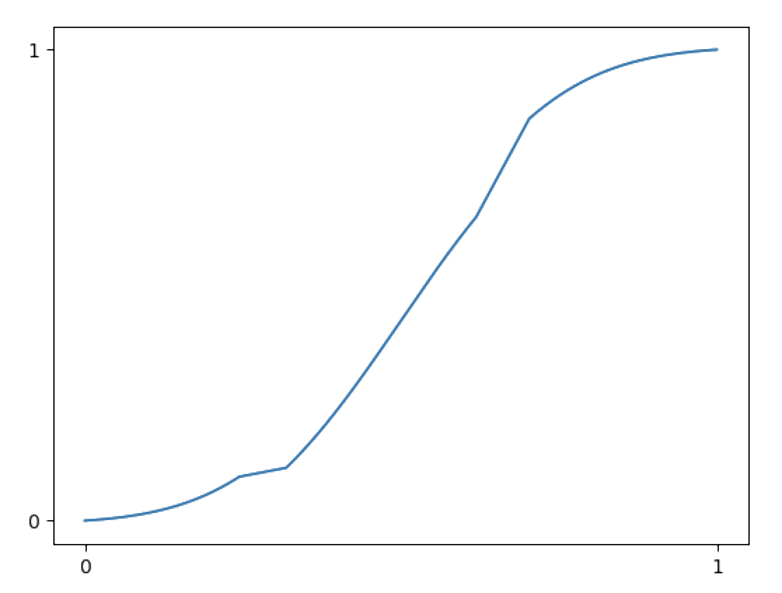
Notice how the test boundaries correspond to cumulative sum elements of the probability distribution? This cumulative sum series is called a CDF - cumulative distribution function. Its value at a certain point, x, represents the probability that a random sample from that distribution will be less than or equal to x.
Inverse sampling the CDF means asking, for a given probability y, at what x does the CDF have a value of y?
Example
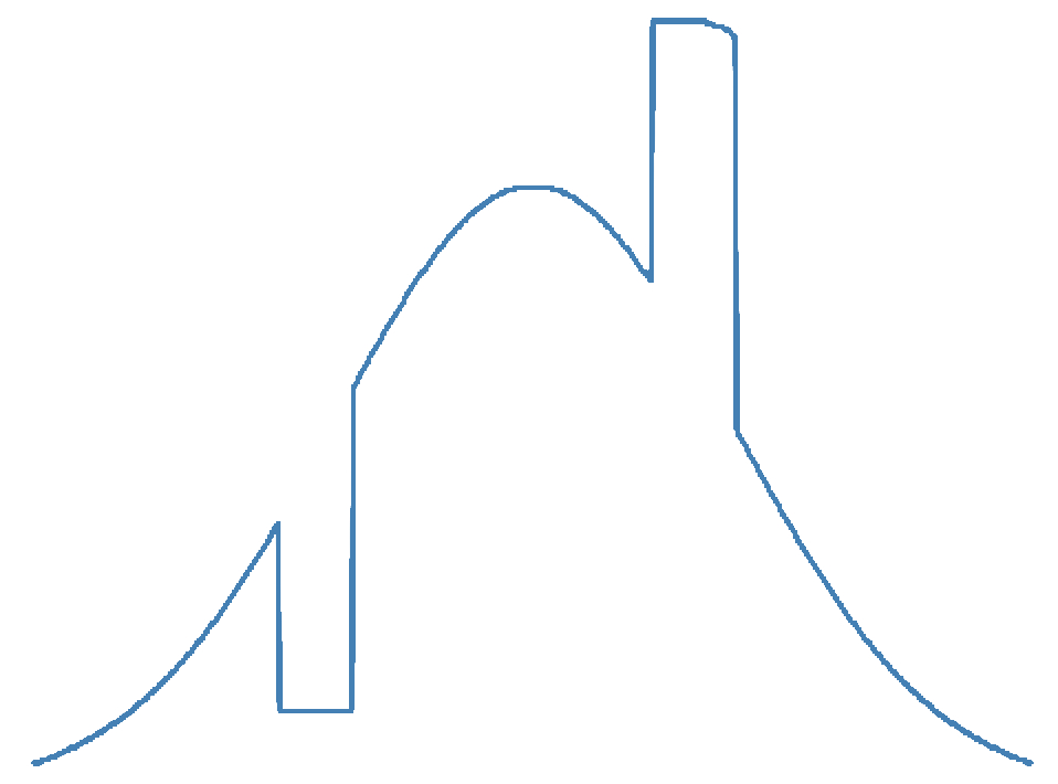
We have this probability distribution:
Then its CDF would be:
To sample a random number from this distribution, we randomly place a horizontal line, and take the x value where it intersects the CDF:
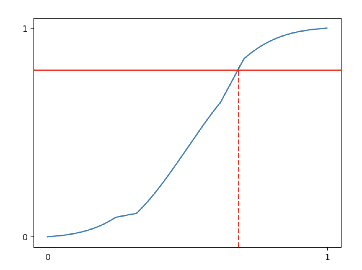
Finding the corresponding x for a sampled probability can be done relatively efficiently (O(logn)) with a binary search, as the CDF is a non-decreasing series.
Effect size and sample size
Choose the “skyline” distribution, and play with the sample size a bit. Try to find, for each skyline feature, the minimum sample size required to distinguish that feature. We see that the smaller the feature is, the larger the sample size required to distinguish that feature.
To me this really illustrates the necessity for large sample sizes when measuring weak effects: when the sample size is too small, the noise is about as large as (or larger than) the effect.
Code for the interactive part of this post can be found here.