Asking the right question

Supervised learning is the machine learning branch that deals with function approximation: using several input-output pairs generated by an unknown target function, construct a different function that approximates the target function. For example, the target function may be my personal movie preferences, and we might be interested in obtaining a model that can predict (approximately) how much I will enjoy watching some new movie. With such a model we can create a movie recommendation app.

Some functions can be easier to approximate than others (given a definition of approximation difficulty, but I won’t go down that rabbit hole right now), and some tasks can be framed as more than one function. This raises the question - do different framings result in different model performance? To find out I tried playing with two framings of a toy problem.

The data

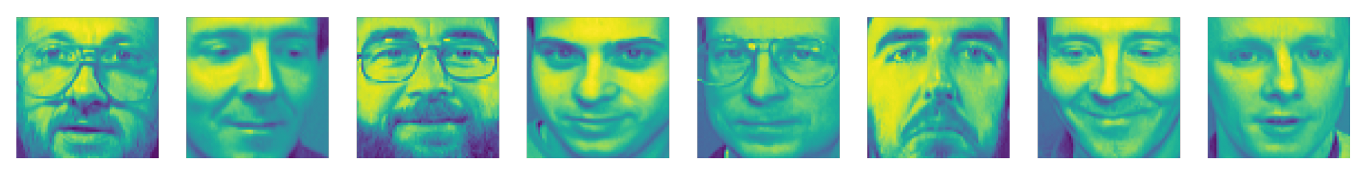
I used the Olivetti faces dataset, which contains grayscale, 64x64 images of the faces of 40 subjects (10 images per subject). Here are some of the faces:

The task

The task is the classical face recognition task (which has been quite controversial lately due to questionable use in settings such as law enforcement). To make things more interesting, I decided to use only two images from each subject for training, and the rest as the test set. So the goal is to train a model which, given an image, outputs the subject that the model believes this face belongs to.

Scope

I wanted to focus just on the aspects of training that pertain to the problem framing, and treat it as a general problem. For that purpose I excluded many specifics that would be very important for a real face recognition application:

• Using existing face recognition models or existing techniques specific to face recognition
• Using data augmentation to generate more training samples
• Obtaining more face data (even without subject information) and perform unsupervised pre-training
• Assigning each prediction a confidence score, and fixing a confidence threshold below which no result is reported

In short, I wanted to see what difference just changing the target function would make. Since the functions are different the models may be somewhat different as well, but they are trained on the same (base) data.

Performance metric

To measure model performance, I used the accuracy metric - percentage of correct classifications. For each framing I ran about 100 train/test splits (with two images in the training set and eight in the test set).

Baseline

As a baseline I used a (single) nearest neighbor classifier with the L2 norm. I.e. when classifying a new face, for each face in the training set we calculate the sum of the squared differences bewteen every two pixels (in similar positions), and take as the answer the face that was closest.

Intuitively it’s hard to tell how well this model would fare. On one hand there should obviously be many similarities between images of the same person (including factors we would have liked to exclude, such as lighting and clothing). On the other hand, many of the similarities we perceive in faces will not be reflected in the pixel-level comparison. In this case the performance (measured as accuracy - percent of correct classifications) of the model was about 70.5%, which is quite impressive in my opinion, considering that a random model would achieve about 2.5% accuracy on average.

Let’s see how a more sophisticated model fares.

First approach

The first framing is the explicit one: given an image, we want to know whose face it is, so that’s what we’ll ask the model. The function maps images to subject identifiers.

For the model I used a simple network with Keras:

model = Sequential([
		Dense(128, input_shape=(X_train.shape[1], ), activation='relu'),
		BatchNormalization(),
		Dense(64, activation='relu'),
		BatchNormalization(),
		Dense(32),
		Dense(y_train.shape[1], activation='softmax')
	])

model.compile(loss='categorical_crossentropy', optimizer='adam')
model.fit(X_train, y_train, epochs=1200)

I played with several variations and this seemed to be the best with regards to number of layers, their sizes and activation functions. Its test accuracy was, on average, about 70.9% - an ever so slight improvement. I think part of the challenge is that classifying faces requires relatively complex features, but we have very little training data (especially considering the number of positive instances for each class). So the model either fails to find a pattern if the network is too small, or overfits if it’s too large.

Second approach

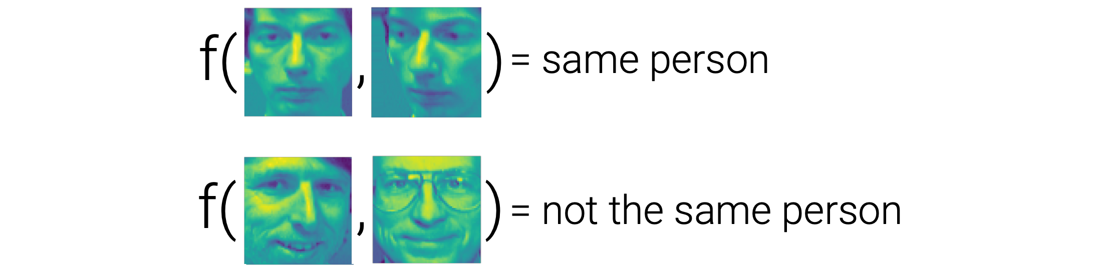
Let’s try a less direct framing. We know that if two images belong to the same person, they should be relatively similar, and vice versa. Therefore, instead of training the model to identify faces, we can train the model to compare faces. In this case, instead of 40 classes (one for every subject) we only have two classes: “same person” or “not the same person”.

Training this model was a little trickier:

• The best architecture turned out to be pretty similar to two (“sideways”) concatenations of the first approach model, which I thought was pretty neat.
• Due to a vanishing gradients issue, I had to go with a slower learning rate and slow it even more as the loss decreased.
• This time we have an imbalanced classification task, so I gave the positive class a bigger weight.
• Training took longer and in a handful of cases (about 5 out of 100) didn’t converge and needed restarting.

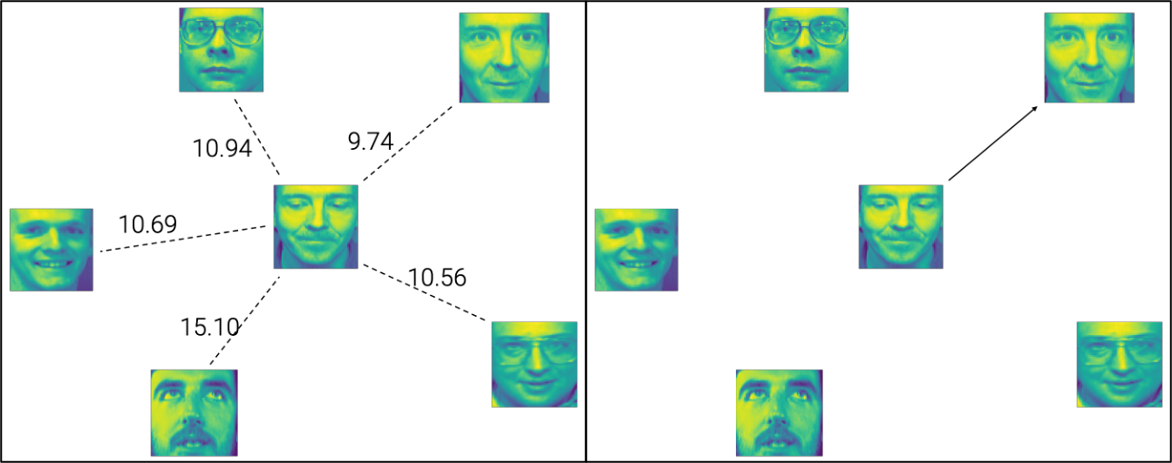
Another difference is that using this framing, inference isn’t straightforward. Instead, we run the model on the input image along with each of the training images, and pick the subject of the image that the model deemed most similar to the input image.

Here is the code for the model and training:

model = Sequential([
		Dense(256, input_shape=(X_train.shape[1], ), activation='relu'),
		BatchNormalization(),
		Dense(128, activation='relu'),
		BatchNormalization(),
		Dense(64),
		BatchNormalization(),
		Dense(2, activation='softmax')
	])

model.compile(loss='categorical_crossentropy', 
	      optimizer=tf.keras.optimizers.Adam(learning_rate=.0001))

for i in range(45):
	hist = model.fit(X_train, to_categorical(y_train),
			 epochs=10, class_weight={0: 1, 1: 79}, verbose=0)
	last_loss = hist.history['loss'][-1]
	lr = .0001
	if last_loss <= .1:
		lr = .00001
	model.compile(loss='categorical_crossentropy',
		      optimizer=tf.keras.optimizers.Adam(learning_rate=lr))

The accuracy of this model was, on average, about 74.4%, which is an improvement over both the first approach and the baseline. However, the spread of the results was larger, resulting in both much worse and much better runs. In this problem, a different framing made quite a significant difference.

Combined approach

After seeing the better average but also bigger spread of the second approach I wondered if it would be possible to create a model that optimizes for both using a non-linear computation graph. The idea was this: each input sample would contain two faces, which would each “go through” several dense layers. The images would be transformed by the same layers separately, and the resulting representation would be used in two ways:

1. Classify each face
2. Concatenate the two representations and, after several more dense layers, classify whether or not they belong to the same person

I also used different weights for the two framings, which worked a little better.

Here’s the code for this model and its training:

x1 = Input(shape=(pre_X_train.shape[1],), name='face1')
x2 = Input(shape=(pre_X_train.shape[1],), name='face2')
L1 = Dense(128, activation='relu', input_shape=(x1.shape[1],), name='face_rep1')
BN1 = BatchNormalization(name='batch_norm1')
L2 = Dense(64, activation='relu', input_shape=(128,), name='face_rep2')
BN2 = BatchNormalization(name='batch_norm2')
L3 = Dense(32, activation='relu', input_shape=(64,), name='face_rep3')
O1 = Dense(40, activation='softmax', input_shape=(32,), name='face_class')

R1 = BN2(L2(BN1(L1(x1))))
R2 = BN2(L2(BN1(L1(x2))))

C1 = concatenate([R1, R2], name='face_rep_concat')
L4 = Dense(64, activation='relu', input_shape=(128,), name='comparison_dense')
BN3 = BatchNormalization(name='batch_norm3')
O2 = Dense(2, activation='softmax', input_shape=(64,), name='comparison_res')

face1_res = O1(L3(R1))
face2_res = O1(L3(R2))
comparison_res = O2(BN3(L4(C1)))

model = Model(inputs=[x1, x2], outputs=[face1_res, face2_res, comparison_res])

tf.keras.utils.plot_model(model, 'model.png', show_shapes=True)

model.compile(optimizer=tf.keras.optimizers.Adam(learning_rate=.0005),
			  loss=[
					tf.keras.losses.categorical_crossentropy,
					tf.keras.losses.categorical_crossentropy,
					weighted_categorical_crossentropy([1, 79]),
			  ],
			  loss_weights=[.05, .05, 1.])

for i in range(130):
	hist = model.fit([X1_train, X2_train], [y1_train, y2_train, y3_train],
			 epochs=10, verbose=0)
	last_loss = hist.history['comparison_res_loss'][-1]
	lr = .0005
	if last_loss <= .5:
		lr = .0001
	if last_loss <= .1:
		lr = .00001

	model.compile(optimizer=tf.keras.optimizers.Adam(learning_rate=lr),
				  loss=[
					  tf.keras.losses.categorical_crossentropy,
					  tf.keras.losses.categorical_crossentropy,
					  weighted_categorical_crossentropy([1, 79]),
				  ],
				  loss_weights=[.05, .05, 1.])

Here’s a visual description of what’s happening:

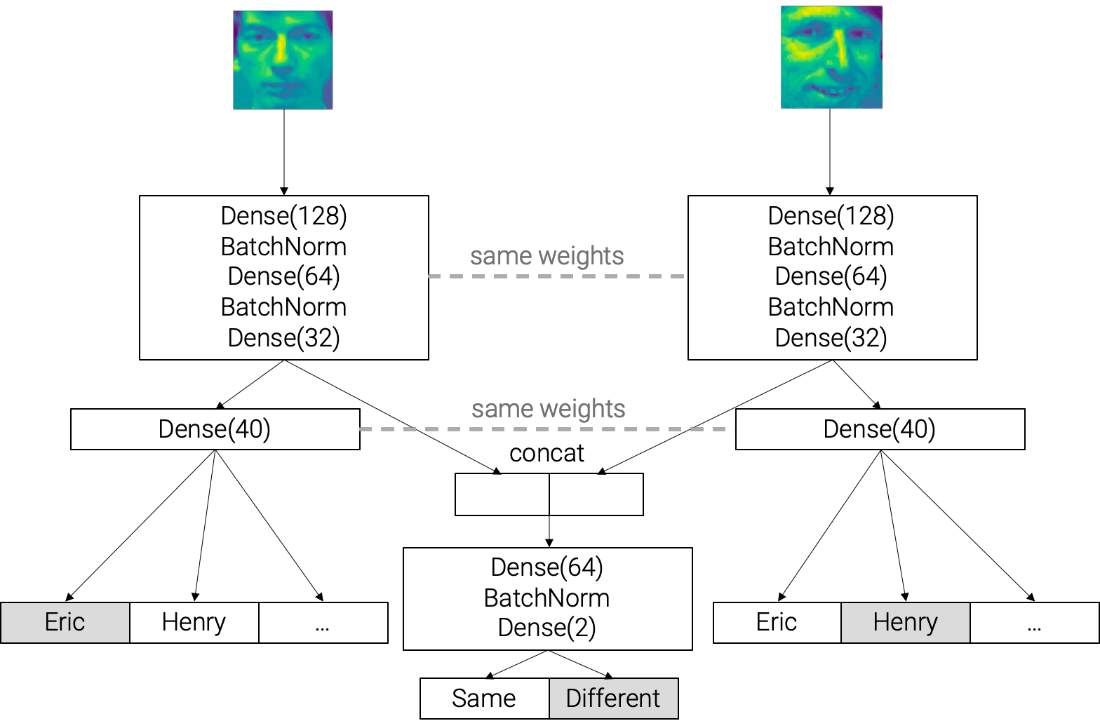
This model took the longest to train. The average accuracy was 73.3%, better than the baseline and the first approach but not as good as the second; however, it was much more stable and there were no incidents of non-convergence. So it seems like the combination indeed enabled us to enjoy both worlds: a little better performance while preserving stability.

Comparison

Model	Description	Mean	Median	5%	95%
Baseline	Nearest neighbor	70.55%	70.625%	65%	76.25%
First approach	Face classification	70.916%	71.094%	65.587%	76.25%
Second approach	Similarity classification	74.381%	75.312%	65.75%	81.9%
Combined approach	first + second	73.328%	73.125%	66.875%	78.656%

Here’s a plot describing the result distributions:

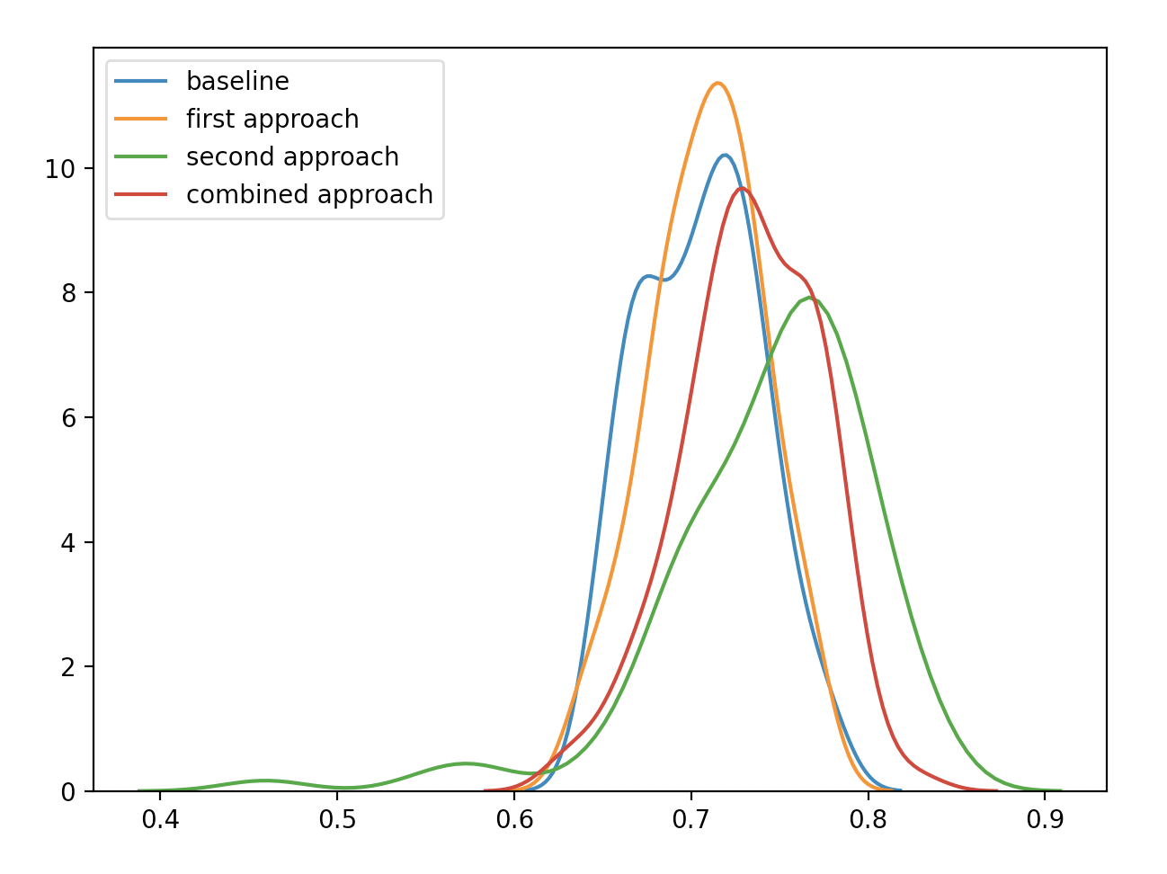
Conclusions

In this instance, framing the task in an alternative, non-straightforward fashion resulted in better model performance.

Bear in mind that this experiment was done on a toy dataset and problem, and the results aren’t necessarily applicable to every problem. However, it highlighted for me the potential in trying out different framings, and going forward I will try to be mindful of alternative framings when I work on supervised tasks.

The source code for this post can be found here. Not as tidy as I would like, but I think it’s clear enough.