Adventures in Imbalanced Learning and Class Weight
Finally turning that stone
A few months ago I was working on an image classification problem with severe class imbalance - the positive class was much rarer than the negative class.
As part of the model tuning phase, I wanted to explore the impact of class imbalance and try to mitigate it. A popular “off-the-shelf” solution to imbalance is weighting classes in inverse proportion to their frequency - which didn’t yield an improvement. This happened to me several times in the past, and other than basic intuition I couldn’t trace the theory of where this weighting comes from (maybe I didn’t try hard enough).
So, I decided to finally try to reason about class weighting in an imbalanced setting from first principles. What follows is my analysis. The TL;DR is that for my problem, I was convinced that class weighting probably doesn’t matter too much.
It’s an interesting analysis and was a fun rabbit-hole to dive into, but makes a lot of assumptions and I’d be careful not to overgeneralize from this.
\(\newcommand{\pipe}{|}\)
The Tradeoff
Wherever there’s a (non-trivial) classification problem, there’s a tradeoff. I’ll focus on the simplest case of binary classification: say we have two classes - negative (denoted 0) and positive (denoted 1); further suppose that the positive is the rare class, with prevalence \(\beta\) (1% in the following visualizations / experiments).
Basically, when we classify, we predict the class of an instance with unknown class. We could be wrong in two ways:
- Classifying a negative instance as positive (false positive)
- Classifying a positive instance as negative (false negative)
It is trivial to avoid making any one type of error: for example, we could classify all instances as negative, avoiding false positives altogether (at the expense of all our positives being false negatives). And therein lies the tradeoff: to make an actual classifier that outputs “hard” predictions, we need to make a product / business decision about how bad each type of error is. Not making an explicit decision means our optimization pipeline has such a choice baked in implicitly.
Now, it’s hard to know in advance how the tradeoff curve will look like. We try to optimize everything else to give us the best set of options: collect lots of data with informative features, use a suitable model, etc. But after all that is done, we still need to choose how to balance the two types of errors.
To optimize this choice in light of our product preferences, we first need to characterize the tradeoff curve.
Characterizing the Tradeoff Curve
Some definitions first:
- We’ll denote \(P(\hat{y} = 1 \pipe y = 1)\) - the probability of predicting a positive given that the instance is positive - as \(x\).
- Similarly, we’ll denote \(P(\hat{y} = 0 \pipe y = 0)\) as \(z\).
For the sake of this analysis I’m going to assume the tradeoff curve is of the form \(z = (1 - x^p) ^ \frac{1}{p}\), with \(p \geq 1\). This yields the following family of curves:
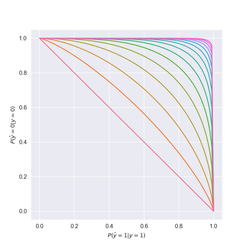
The red curve corresponds to \(p = 1\) - a pretty poor tradeoff curve. As we increase \(p\), our set of options improves. At the coveted (but realistically unattainable) \(p = \infty\) we’d choose \(x = z = 1\), beat the problem altogether and go home; until then, we have to choose some compromise between \(x\) and \(z\).
Later, we’ll ponder how to choose the tradeoff. But to do that we first need to define what it is we’re even trying to optimize.
Taking a Stance
Like I previously mentioned, initial modeling stages try to give us the best tradeoff curve possible for the task - using data, model type, training techniques, whatever. At those stages we can optimize for threshold-independent metrics, for example various area under the curve metrics. But ultimately, somewhere downstream the model’s output will be binarized, and we might as well take that into consideration when tuning the model.
I’m personally fond of the F-score - it combines two very interpretable metrics (precision and recall), which makes communicating with less technical stakeholders (such as product managers and the FDA) easier, and can be easily tweaked to account for error type preferences.
For this problem precision and recall were equally important, so I used the \(F_1\) score:
\[F_1 = \frac{2}{\frac{1}{precision} + \frac{1}{recall}}\]Ultimately, this is the metric we want to optimize.
Where’s the Knob?
OK, so we know what we want to optimize, and we know that our choices are limited by the tradeoff curve. But how do we control where we land on the curve?
Canonically, binary classification is framed as minimizing binary cross-entropy loss. The knob we’ll use to decide where we land on the tradeoff curve is a weighting coefficient, \(\alpha\), for the positive instances:
\[BCE = -\sum_i{\alpha y_i \log_2{\hat{y_i}} + (1 - y_i) \log_2{(1 - \hat{y_i}}))}\]Optimizing Away
Now that all the actors are on stage, let’s roll up our sleeves and get our hands dirty.
First, we’ll take a step back from looking at individual instances, and look at the relationship between positive and negative instances, based on \(\beta\), the positive class prevalence. To that end, we’ll replace individual \(\hat{y_i}\) and \(1 - \hat{y_i}\) with their respective expectations, \(x\) and \(z\). Further, our assumed tradeoff curve constrains one by the other; let’s reframe the loss as a function of \(x\) (also dependent on \(\alpha\), \(\beta\), and \(p\).)
\[BCE(x) = -(\alpha \beta \log{x} + (1 - \beta)\frac{\log{(1 - x^p)}}{p})\]We’ll now differentiate wrt \(x\) to find where on the tradeoff curve our choice of \(\alpha\) and the reality of \(\beta\) and \(p\) have landed us:
\[BCE'(x) = -(\frac{\alpha \beta}{x \ln{2}} + \frac{1 - \beta}{p} \cdot \frac{1}{(1 - x^p) \ln{2}} \cdot (-p x ^ {p - 1})) =\] \[= \frac{(1 - \beta) x ^ {p - 1}}{(1 - x ^ p)\ln{2}} - \frac{\alpha \beta}{x \ln{2}}\] \[BCE'(x) = 0 \Leftrightarrow (1 - \beta)x ^ p = \alpha \beta (1 - x^p)\]And we finally get:
\[x = \sqrt[p]{\frac{\alpha \beta}{\alpha \beta - \beta + 1}}\]Halftime recap
We’ve been handed a binary classification problem characterized by \(\beta\) and \(p\). We optimized a classifier using weighted binary cross-entropy with weight \(\alpha\) for the positive, rare class. This lands us in a particular place on the tradeoff curve, which we just found (these are \(x\) and \(z\)).
Next, we’ll want to see how our choice of \(\alpha\) trickles downstream to the \(F_1\) score, and use this description to find an optimal value for \(\alpha\).
Calculating \(F_1\)
We’re interested in calculating the expected \(F_1\) score resulting from our choice of \(\alpha\). Since \(F_1\) depends directly on precision and recall, we’ll calculate the expected value of those metrics.
Recall is easy - it is the fraction of positive instances we correctly detected as positive, and we can expect it to be \(x\) - the probability our classifier outputs 1 for a positive instance.
Precision is the fraction \(\frac{true \ positives}{true \ positives + false \ positives}\).
The expected true positives are the fraction of positives times the probability of detecting a positive as such: \(\beta x\).
The expected false positives are the negative instances which were misclassified: \((1 - \beta)(1 - z)\).
Putting all that in the \(F_1\) formula:
\[\mathbb{E}(F_1) = \frac{2}{\frac{\beta x + (1 - \beta)(1 - z)}{\beta x} + \frac{1}{x}} = \frac{2 \beta x}{\beta x + \beta z + 1 - z}\]While \(\alpha\) does not explicitly appear here, it’s part of \(x\) and \(z\) which we know and do appear here.
Great! So all that’s left is differentiating wrt \(\alpha\) and finding the maximum, right?
\[\tiny{\frac{2 \beta \left(\frac{\alpha \beta}{\alpha \beta - \beta + 1}\right)^{\frac{1}{p}} \left(\left(1 - \beta\right) \left(\left(\left(\frac{\alpha \beta}{\alpha \beta - \beta + 1}\right)^{\frac{1}{p}}\right)^{p} - 1\right)^{2} \left(\beta \left(\frac{\alpha \beta}{\alpha \beta - \beta + 1}\right)^{\frac{1}{p}} + \beta \left(1 - \left(\left(\frac{\alpha \beta}{\alpha \beta - \beta + 1}\right)^{\frac{1}{p}}\right)^{p}\right)^{\frac{1}{p}} - \left(1 - \left(\left(\frac{\alpha \beta}{\alpha \beta - \beta + 1}\right)^{\frac{1}{p}}\right)^{p}\right)^{\frac{1}{p}} + 1\right) + \left(\beta - 1\right) \left(\beta \left(\frac{\alpha \beta}{\alpha \beta - \beta + 1}\right)^{\frac{1}{p}} \left(\left(\left(\frac{\alpha \beta}{\alpha \beta - \beta + 1}\right)^{\frac{1}{p}}\right)^{p} - 1\right)^{2} - \beta \left(1 - \left(\left(\frac{\alpha \beta}{\alpha \beta - \beta + 1}\right)^{\frac{1}{p}}\right)^{p}\right)^{\frac{p + 1}{p}} \left(\left(\frac{\alpha \beta}{\alpha \beta - \beta + 1}\right)^{\frac{1}{p}}\right)^{p} + \left(1 - \left(\left(\frac{\alpha \beta}{\alpha \beta - \beta + 1}\right)^{\frac{1}{p}}\right)^{p}\right)^{\frac{p + 1}{p}} \left(\left(\frac{\alpha \beta}{\alpha \beta - \beta + 1}\right)^{\frac{1}{p}}\right)^{p}\right)\right)}{\alpha p \left(\left(\left(\frac{\alpha \beta}{\alpha \beta - \beta + 1}\right)^{\frac{1}{p}}\right)^{p} - 1\right)^{2} \left(\alpha \beta - \beta + 1\right) \left(\beta \left(\frac{\alpha \beta}{\alpha \beta - \beta + 1}\right)^{\frac{1}{p}} + \beta \left(1 - \left(\left(\frac{\alpha \beta}{\alpha \beta - \beta + 1}\right)^{\frac{1}{p}}\right)^{p}\right)^{\frac{1}{p}} - \left(1 - \left(\left(\frac{\alpha \beta}{\alpha \beta - \beta + 1}\right)^{\frac{1}{p}}\right)^{p}\right)^{\frac{1}{p}} + 1\right)^{2}}}\]Uh, haha, never mind, let’s do that numerically.
Here is a plot of the expected \(F_1\) as a function of \(\alpha\) for a range of values for \(p\).
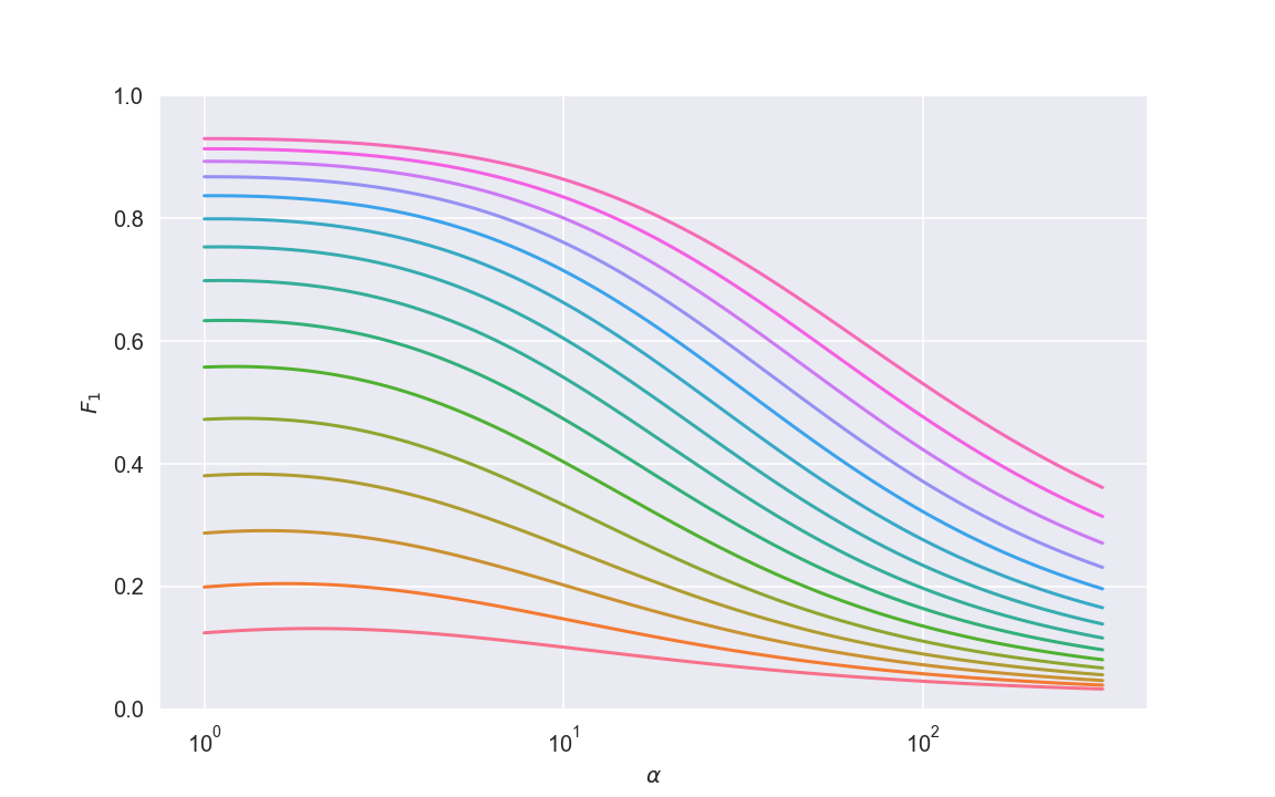
The red curve corresponds to \(p \approx 2\), and shows pretty abysmal results; as \(p\) increases, we get better and better results.
The range of \(\alpha\) goes from 1 (which is equivalent to unweighted training) to about 250, with 100 being the “inverse proportion” weighting practice.
Most prominently, what we see is that class weight hardly improves over unweighted training, and the optimal weight is usually only a bit larger than the unweighted version, and far from the inverse proportion. In fact, from these plots, it would seem that using the inverse proportion weighting scheme is actually detrimental to training!
Very interesting indeed.
Caveats and Limitations
This is a good place to remember that we made a lot of assumptions to get here. Several things in particular may limit the scope of the conclusions:
- Assuming a completely symmetric tradeoff curve
- Assuming no label noise in training
- Assigning equal importance to precision and recall
Sanity Check
I wanted to get a sense for the generalizability of the conclusions outside the sterile mathematical environment. I set up a rudimentary imbalanced classification pipeline with scikit-learn’s make_classification and DecisionTreeClassifier, and created an empirical version of the above plot, using class_sep as a proxy for the tradeoff curve.
A couple of things in that setup are different enough from my clean assumptions that I was very curious to see the results. I let my computer crunch for a few hours (running hundreds of thousands of simulations) and it produced the following plot:
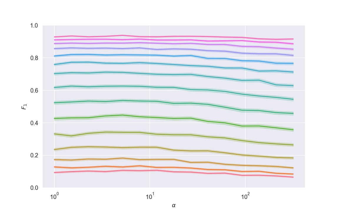
Nice! It’s not identical to the theory-derived plot, but looks very similar, and in particular:
- The optimal weight is only slightly larger than 1, but
- It doesn’t really matter anyway - the optimal weight only gives a negligible performance boost
As for why the plot looks different for bigger values of \(\alpha\), my hunch is that the tradeoff curve isn’t symmetric, allowing the classifier to get a decent recall without sacrificing precision entirely.
Conclusions
While I certainly don’t know everything about class weighting now, I’ve come away from the analysis very satisfied: I know that class imbalance, in and of itself, does not warrant using class weights. Furthermore, if I deem class weights necessary, instead of using the typical “inverse proportion” scheme, my weights had better be informed by the particular problem characteristics: the nature of the tradeoff curve, label noise, and the cost I assign to each type of error.
Update 08/05/2025
After publishing the post it’s been pointed out to me that there are tutorials that specifically demonstrate how inverse proportion weighting (or stratified under- / oversampling, which is pretty equivalent) improves imbalanced classification performance. This piqued my interest and I looked at such a tutorial, and found something very interesting. To measure performance, the tutorial used the balanced accuracy score rather than \(F_1\).
\(F_1\) is the harmonic average of positive precision and positive recall; balanced accuracy is the (regular) average between positive recall and negative recall. On the surface, the two metrics look similar enough: each in itself is a combination of two metrics, corresponding to the two types of errors we can make.
But, as always, the details are important. I used the same optimization framework as before but looked at expected balanced accuracy (instead of expected \(F_1\)) as a function of class weight, and here’s what I got:
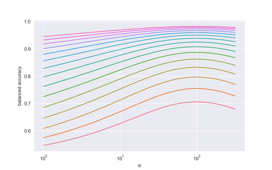
Look at that - completely different from the \(F_1\) behavior! Moreover, the optimal weight is indeed the inverse proportion rule of thumb. This is splendid: the theoretic methodology is in accordance with results people get in the wild. Less selfishly, it really highlights the importance of choice of metric on model tuning - different metrics respond very differently to our choice of hyperparameters.
\(F_1\) vs. balanced accuracy
Let’s dive into the difference between the two metrics, so we have an intuition for which one to choose. Specifically, we’ll look for a scenario where they are very different from each other.
Imagine we have 1000 samples - 10 positive, 990 negative. We classify all positives as positive, 40 negatives as positive. Positive recall is perfect (100%), negative recall is \(\frac{950}{990} \approx\) 96%, positive precision is \(\frac{10}{50} =\) 20%. Balanced accuracy would be very high, but \(F_1\) would be very low.
This is an example of the way different metrics induce different preferences over the two types of errors. There’s no absolute right or wrong here - it’s a matter of aligning your technical choice to the domain.
Conclusion (again)
To me, this reinforces the importance of considering the downstream use of the model, and consulting business stakeholders when tuning the model for hard prediction.
Code
Code for the visualizations and simulation can be found here.
Related
- Cost-sensitive machine learning
- Classifier Calibration
- In particular this PyCon talk from core
scikit-learn(and previouslyimbalanced-learn) developer
- In particular this PyCon talk from core